Independent research · 2025 to 2026 · Sole author

The Geometry of Risk

A four-layer monitoring framework that reads systemic stress in the structure of nine global asset classes: how tightly they move together, who leads whom, how fat the tails are, and which regime the market is in.

MethodsPCA / Absorption RatioCorrelation networks (MST)Granger causality + BonferroniVAR / variance decompositionCVaR, tail dependenceDCC-GARCHGaussian HMM, out-of-sample ToolsPythonpandasstatsmodelsscikit-learnhmmlearnarchnetworkx DomainSystemic risk monitoring · multi-asset portfolios · financial econometrics

4 of 4

crisis windows breach the 0.50 Absorption Ratio threshold

4 of 72

directional Granger links survive Bonferroni correction, all into Japan Equity

Apr 2026

stress flagged by an HMM trained on 2011 to March 2025 and never refitted

Read the paper (SSRN) Code and data DOI 10.2139/ssrn.7521018

The problem

Diversification fails exactly when it's needed. In a crisis, assets that usually move independently start moving as one block, and a single correlation number hides it. I wanted a monitor that reads the structure of the market directly, and that a risk team could reproduce.

Data

Universe	9 asset classes: US, EU, Japan, China and emerging-market equity; gold; oil; the US dollar index; the US 10-year yield
Study window	24 Apr 2025 to 24 Apr 2026 · N = 261 trading days
Long history	2011 to 2026 · N = 3,472 trading days
Sources	Yahoo Finance prices; FRED CPI and 10-year yield; a frozen snapshot is committed to the repo

Approach

Network topology. Turn correlations into distances, then map the market with a minimum spanning tree, multidimensional scaling and Ward clustering.
Causality. Test all 72 directed pairs for Granger causality, keep only what survives Bonferroni correction, and cross-check with joint F-tests and variance decomposition in a nine-asset VAR.
Tail risk. Measure CVaR and lower-tail dependence directly instead of trusting variance.
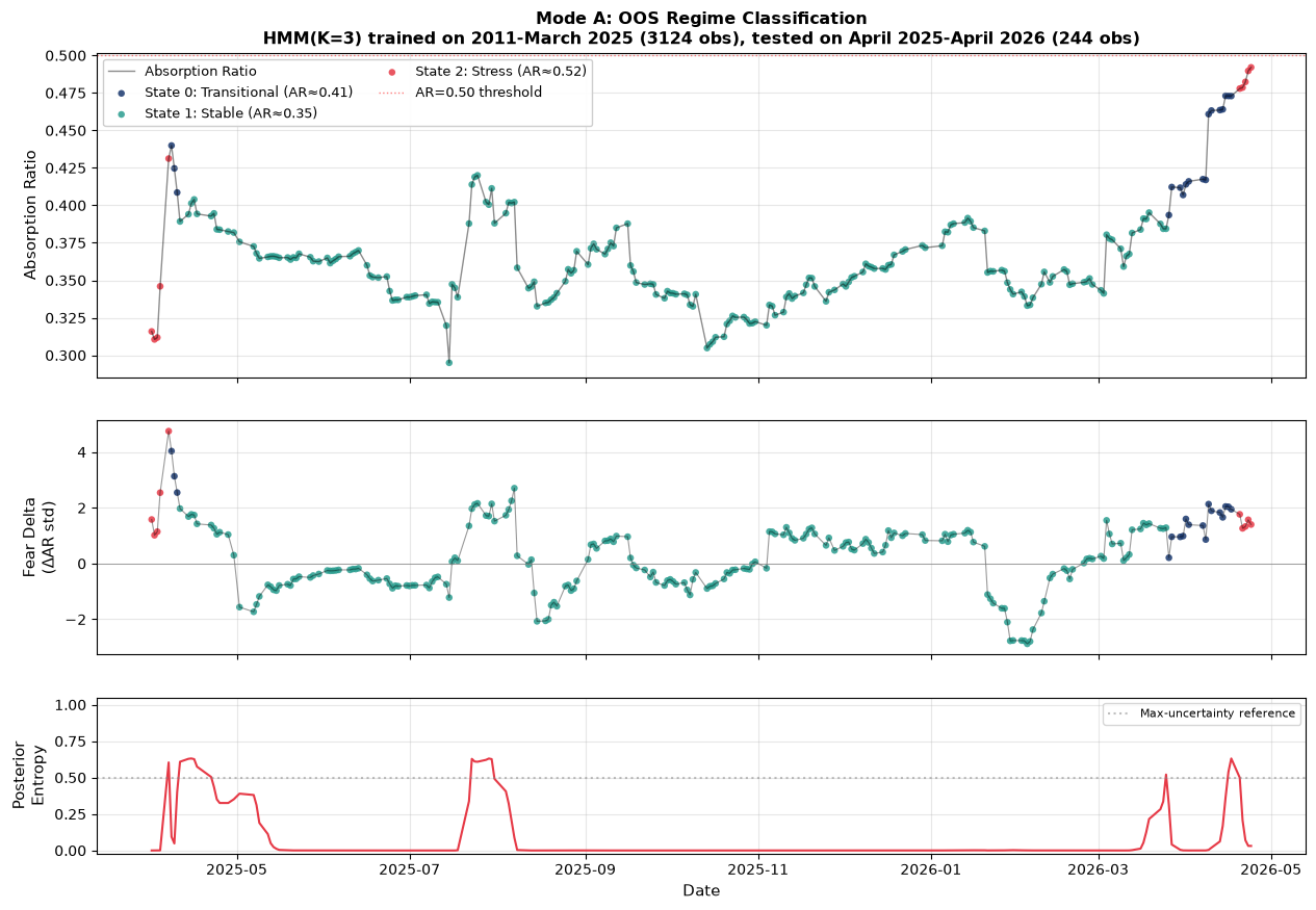
Regimes. Track the Absorption Ratio against the 0.50 threshold of Kritzman et al. (2011), and classify regimes with a Gaussian HMM trained on 2011 to March 2025, then applied to the next year without refitting.

Results

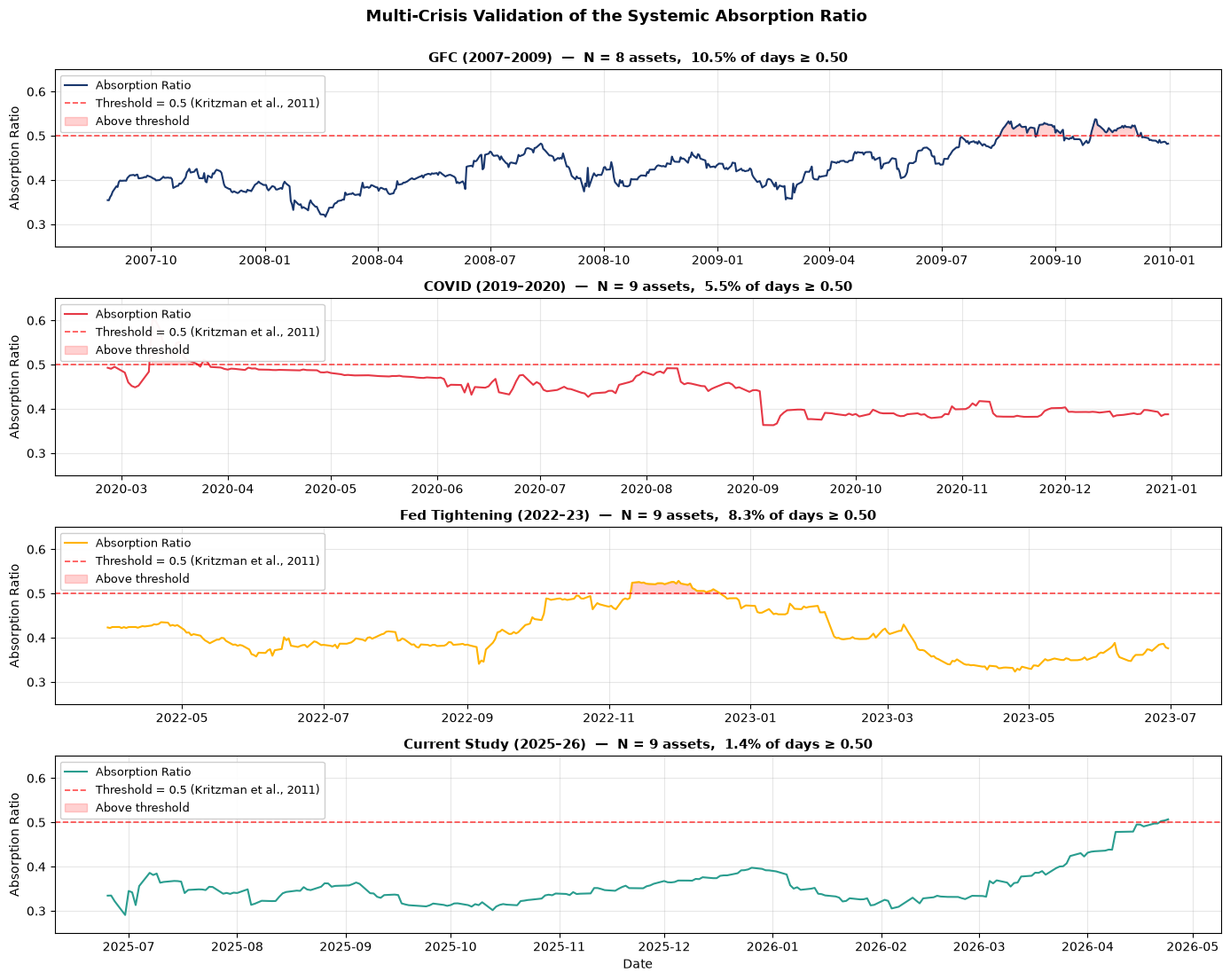
Absorption Ratio in four stress episodes, each crossing the 0.50 threshold — **Figure 1.** The Absorption Ratio crosses 0.50 in all four episodes: GFC peak 0.537, COVID 0.601, Fed tightening 0.529, the 2025–26 study window 0.507. Source

The current-study breach is brief and marginal, 3 days at the very end of the window. That's why the other three layers matter.

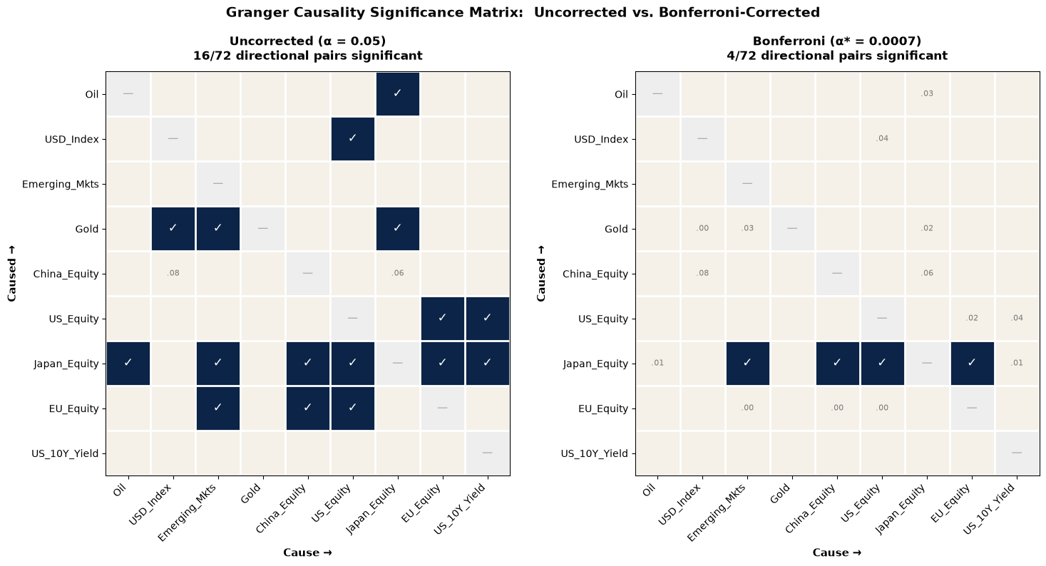
Granger causality matrix before and after Bonferroni correction — **Figure 2.** Of 72 directed pairs, 4 survive the Bonferroni threshold (α* = 0.0007): US, EU, China and emerging-market equity each lead Japanese equity. Source

Out-of-sample HMM regime probabilities over the study year — **Figure 3.** Out of sample, the HMM labels 4.1% of the year as stress (its training base rate was 25.6%), in two episodes: the April 2025 tariff shock and the April 2026 peak. Source

Two more findings: the correlation-network tree and a parametric DCC-GARCH tree share 5 of 8 links, and oil is quasi-exogenous in the conditional mean (joint F-test p = 0.38 and 0.33) while still explaining 11–16% of the 10-day forecast-error variance of EU equity, emerging markets and the 10-year yield.

Live dashboard

The framework's core layer, refitted on current market data. It shows the tool running; the paper's results come from the fixed, out-of-sample-validated model in the repo.

Rolling Absorption Ratio · 60-day window, regime-shaded

CalmTransitionalStressDashed line: 0.50 threshold (Kritzman et al., 2011)

Accelerator · standardised 15-day change in the Absorption Ratio

Above +2σ: risk building fastBelow −2σ: risk easing fast

Correlation matrix · trailing 60 trading days

Data: Yahoo Finance, 9 assets. PCA from scikit-learn; 3-state Gaussian HMM from hmmlearn, refitted on each update. Generated .

Limitations

261 trading days is short for systemic-risk work, so findings specific to this window are exploratory.
Granger tests assume linear dependence; only Bonferroni-robust links are treated as solid.
Next steps: walk-forward HMM evaluation, non-linear causality (transfer entropy) and copula-based tail dependence.

Reproduce it

git clone https://github.com/youness-yach/geometry-of-risk
pip install -r requirements.txt
jupyter nbconvert --to notebook --execute notebooks/geometry_of_risk.ipynb

The repo runs on the frozen study window, so every run gives the same result. A few secondary figures differ slightly from the paper, which used a live download in May 2026; the repo documents each difference.